5.5 Calculating Electric Fields of Charge Distributions

The charge distributions we have seen so far have been discrete: made up of individual point particles. This is in contrast with a continuous charge distribution, which has at least one nonzero dimension. If a charge distribution is continuous rather than discrete, we can generalize the definition of the electric field. We simply divide the charge into infinitesimal pieces and treat each piece as a point charge.

Note that because charge is quantized, there is no such thing as a “truly” continuous charge distribution. However, in most practical cases, the total charge creating the field involves such a huge number of discrete charges that we can safely ignore the discrete nature of the charge and consider it to be continuous. This is exactly the kind of approximation we make when we deal with a bucket of water as a continuous fluid, rather than a collection of ${\text{H}}_2\text{O}$ molecules.

Our first step is to define a charge density for a charge distribution along a line, across a surface, or within a volume, as shown in Figure 5.22.

Figure 5.22 The configuration of charge differential elements for (a) a line charge, (b) a sheet of charge, and (c) a volume of charge. Also note that (d) some of the components of the total electric field cancel out, with the remainder resulting in a net electric field.

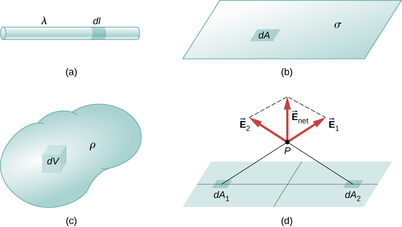
Definitions of charge density:

• $\lambda \equiv$ charge per unit length (linear charge density); units are coulombs per meter (C/m)
• $\sigma \equiv$ charge per unit area (surface charge density); units are coulombs per square meter $(\text{C}\text{/}{\text{m}}^2)$
• $\rho \equiv$ charge per unit volume (volume charge density); units are coulombs per cubic meter $(\text{C}\text{/}{\text{m}}^3)$

Then, for a line charge, a surface charge, and a volume charge, the summation in Equation 5.4 becomes an integral and $q_i$ is replaced by $dq=\lambda dl$, $\sigma dA$, or $\rho dV$, respectively:

The integrals are generalizations of the expression for the field of a point charge. They implicitly include and assume the principle of superposition. The “trick” to using them is almost always in coming up with correct expressions for dl, dA, or dV, as the case may be, expressed in terms of r, and also expressing the charge density function appropriately. It may be constant; it might be dependent on location.

Note carefully the meaning of r in these equations: It is the distance from the charge element $\left(q_i,\lambda dl,\sigma dA,\rho dV\right)$ to the location of interest, $P\left(x,y,z\right)$ (the point in space where you want to determine the field). However, don’t confuse this with the meaning of $\widehat{\text{r}}$; we are using it and the vector notation $\overrightarrow{\text{E}}$ to write three integrals at once. That is, Equation 5.9 is actually

Example 5.5

Electric Field of a Line Segment

Find the electric field a distance z above the midpoint of a straight line segment of length L that carries a uniform line charge density $\lambda$.

Strategy

Since this is a continuous charge distribution, we conceptually break the wire segment into differential pieces of length dl, each of which carries a differential amount of charge $dq=\lambda dl$. Then, we calculate the differential field created by two symmetrically placed pieces of the wire, using the symmetry of the setup to simplify the calculation (Figure 5.23). Finally, we integrate this differential field expression over the length of the wire (half of it, actually, as we explain below) to obtain the complete electric field expression.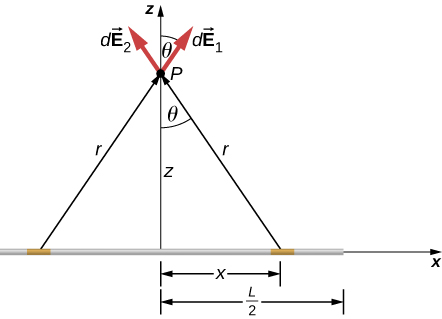

Figure 5.23 A uniformly charged segment of wire. The electric field at point P can be found by applying the superposition principle to symmetrically placed charge elements and integrating.

Solution

Before we jump into it, what do we expect the field to “look like” from far away? Since it is a finite line segment, from far away, it should look like a point charge. We will check the expression we get to see if it meets this expectation.

The electric field for a line charge is given by the general expression

$$\overrightarrow{\text{E}}\left(P\right)=\frac{1}{4\pi {\epsilon }_0}{\displaystyle {\int }_{\text{line}}\frac{\lambda dl}{r^2}}\widehat{\text{r}}.$$

The symmetry of the situation (our choice of the two identical differential pieces of charge) implies the horizontal (x)-components of the field cancel, so that the net field points in the z-direction. Let’s check this formally.

The total field $\overrightarrow{\text{E}}\left(P\right)$ is the vector sum of the fields from each of the two charge elements (call them ${\overrightarrow{\text{E}}}_1$ and ${\overrightarrow{\text{E}}}_2$, for now):

$$\overrightarrow{\text{E}}\left(P\right)={\overrightarrow{\text{E}}}_1+{\overrightarrow{\text{E}}}_2=E_{1x}\widehat{\text{i}}+E_{1z}\widehat{\text{k}}+E_{2x}\left(\text{−}\widehat{\text{i}}\right)+E_{2z}\widehat{\text{k}}.$$

Because the two charge elements are identical and are the same distance away from the point P where we want to calculate the field, $E_{1x}=E_{2x},$ so those components cancel. This leaves

$$\overrightarrow{\text{E}}\left(P\right)=E_{1z}\widehat{\text{k}}+E_{2z}\widehat{\text{k}}=E_1\text{cos}\theta \widehat{\text{k}}+E_2\text{cos}\theta \widehat{\text{k}}.$$

These components are also equal, so we have

$$\begin{array}{cc}\hfill \overrightarrow{\text{E}}\left(P\right)& =\frac{1}{4\pi {\epsilon }_0}{\displaystyle \int \frac{\lambda dl}{r^2}}\text{cos}\theta \widehat{\text{k}}+\frac{1}{4\pi {\epsilon }_0}{\displaystyle \int \frac{\lambda dl}{r^2}}\text{cos}\theta \widehat{\text{k}}\hfill \\ & =\frac{1}{4\pi {\epsilon }_0}{\displaystyle {\int }_0^{L\text{/}2}\frac{2\lambda dx}{r^2}}\text{cos}\theta \widehat{\text{k}}\hfill \end{array}$$

where our differential line element dl is dx, in this example, since we are integrating along a line of charge that lies on the x-axis. (The limits of integration are 0 to $\frac{L}{2}$, not $-\frac{L}{2}$ to $+\frac{L}{2}$, because we have constructed the net field from two differential pieces of charge dq. If we integrated along the entire length, we would pick up an erroneous factor of 2.)

In principle, this is complete. However, to actually calculate this integral, we need to eliminate all the variables that are not given. In this case, both r and $\theta$ change as we integrate outward to the end of the line charge, so those are the variables to get rid of. We can do that the same way we did for the two point charges: by noticing that

$$r={\left(z^2+x^2\right)}^{1\text{/}2}$$

and

$$\text{cos}\theta =\frac{z}{r}=\frac{z}{{\left(z^2+x^2\right)}^{1\text{/}2}}.$$

Substituting, we obtain

$$\begin{array}{cc}\hfill \overrightarrow{\text{E}}\left(P\right)& =\frac{1}{4\pi {\epsilon }_0}{\displaystyle {\int }_0^{L\text{/}2}\frac{2\lambda dx}{\left(z^2+x^2\right)}}\frac{z}{{\left(z^2+x^2\right)}^{1\text{/}2}}\widehat{\text{k}}\hfill \\ & =\frac{1}{4\pi {\epsilon }_0}{\displaystyle {\int }_0^{L\text{/}2}\frac{2\lambda z}{{\left(z^2+x^2\right)}^{3\text{/}2}}}dx\widehat{\text{k}}\hfill \\ & =\frac{2\lambda z}{4\pi {\epsilon }_0}\left[\frac{x}{z^2\sqrt{z^2+x^2}}\right]{|}_0^{L\text{/}2}\widehat{\text{k}}\hfill \end{array}$$

which simplifies to

$$\overrightarrow{\text{E}}(z)=\frac{1}{4\pi {\epsilon }_0}\frac{\lambda L}{z\sqrt{z^2+\frac{L^2}{4}}}\widehat{\text{k}}.$$

5.12

Significance

Notice, once again, the use of symmetry to simplify the problem. This is a very common strategy for calculating electric fields. The fields of nonsymmetrical charge distributions have to be handled with multiple integrals and may need to be calculated numerically by a computer.

In the case of a finite line of charge, note that for $z\gg L$, $z^2$ dominates the L in the denominator, so that Equation 5.12 simplifies to

If you recall that $\lambda L=q$, the total charge on the wire, we have retrieved the expression for the field of a point charge, as expected.

In the limit $L\to \infty$, on the other hand, we get the field of an infinite straight wire, which is a straight wire whose length is much, much greater than either of its other dimensions, and also much, much greater than the distance at which the field is to be calculated:

An interesting artifact of this infinite limit is that we have lost the usual $1\text{/}{r}^2$ dependence that we are used to. This will become even more intriguing in the case of an infinite plane.

Example 5.7

Electric Field due to a Ring of Charge

A ring has a uniform charge density $\lambda$, with units of coulomb per unit meter of arc. Find the electric field at a point on the axis passing through the center of the ring.

Strategy

We use the same procedure as for the charged wire. The difference here is that the charge is distributed on a circle. We divide the circle into infinitesimal elements shaped as arcs on the circle and use polar coordinates shown in Figure 5.24.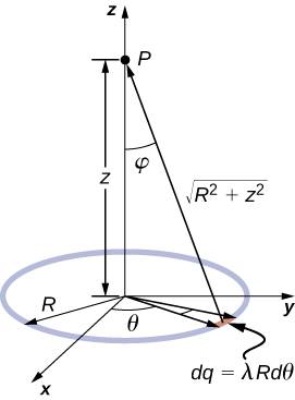

Figure 5.24 The system and variable for calculating the electric field due to a ring of charge.

Solution

The electric field for a line charge is given by the general expression

$$\overrightarrow{\text{E}}\left(P\right)=\frac{1}{4\pi {\epsilon }_0}{\displaystyle {\int }_{\text{line}}\frac{\lambda dl}{r^2}}\widehat{\text{r}}.$$

A general element of the arc between $\theta$ and $\theta +d\theta$ is of length $Rd\theta$ and therefore contains a charge equal to $\lambda Rd\theta .$ The element is at a distance of $r=\sqrt{z^2+R^2}$ from P, the angle is $\text{cos}\varphi =\frac{z}{\sqrt{z^2+R^2}}$, and therefore the electric field is

$$\begin{array}{cc}\overrightarrow{\text{E}}\left(P\right)\hfill & =\frac{1}{4\pi {\epsilon }_0}{\displaystyle {\int }_{\text{line}}\frac{\lambda dl}{r^2}}\widehat{\text{r}}=\frac{1}{4\pi {\epsilon }_0}{\displaystyle {\int }_0^{2\pi }\frac{\lambda Rd\theta }{z^2+R^2}\frac{z}{\sqrt{z^2+R^2}}\widehat{z}}\hfill \\ & =\frac{1}{4\pi {\epsilon }_0}\frac{\lambda Rz}{{\left(z^2+R^2\right)}^{3\text{/}2}}\widehat{z}{\displaystyle {\int }_0^{2\pi }d\theta }=\frac{1}{4\pi {\epsilon }_0}\frac{2\pi \lambda Rz}{{\left(z^2+R^2\right)}^{3\text{/}2}}\widehat{z}\hfill \\ & =\frac{1}{4\pi {\epsilon }_0}\frac{q_{\text{tot}}z}{{\left(z^2+R^2\right)}^{3\text{/}2}}\widehat{z}.\hfill \end{array}$$

Significance

As usual, symmetry simplified this problem, in this particular case resulting in a trivial integral. Also, when we take the limit of $z>>R$, we find that

$$\overrightarrow{\text{E}}\approx \frac{1}{4\pi {\epsilon }_0}\frac{q_{\text{tot}}}{z^2}\widehat{z},$$

as we expect.

Example 5.8

The Field of a Disk

Find the electric field of a circular thin disk of radius R and uniform charge density at a distance z above the center of the disk (Figure 5.25)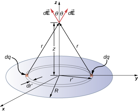

Figure 5.25 A uniformly charged disk. As in the line charge example, the field above the center of this disk can be calculated by taking advantage of the symmetry of the charge distribution.

Strategy

The electric field for a surface charge is given by

$$\overrightarrow{\text{E}}(P)=\frac{1}{4\pi {\epsilon }_0}{\displaystyle {\int }_{\text{surface}}\frac{\sigma dA}{r^2}}\widehat{\text{r}}.$$

To solve surface charge problems, we break the surface into symmetrical differential “strips” that match the shape of the surface; here, we’ll use rings, as shown in the figure. Again, by symmetry, the horizontal components cancel and the field is entirely in the vertical $(\widehat{\text{k}})$ direction. The vertical component of the electric field is extracted by multiplying by $\text{cos}\theta$, so

$$\overrightarrow{\text{E}}(P)=\frac{1}{4\pi {\epsilon }_0}{\displaystyle {\int }_{\text{surface}}\frac{\sigma dA}{r^2}}\text{cos}\theta \widehat{\text{k}}.$$

As before, we need to rewrite the unknown factors in the integrand in terms of the given quantities. In this case,

$$\begin{array}{ccc}\hfill dA& =\hfill & 2\pi r^{\text{′}}d{r}^{\prime }\hfill \\ \hfill r^2& =\hfill & {r^{\prime }}^2+z^2\hfill \\ \hfill \text{cos}\theta & =\hfill & \frac{z}{{\left({r^{\prime }}^2+z^2\right)}^{1\text{/}2}}.\hfill \end{array}$$

(Please take note of the two different “r’s” here; r is the distance from the differential ring of charge to the point P where we wish to determine the field, whereas $r^{\prime }$ is the distance from the center of the disk to the differential ring of charge.) Also, we already performed the polar angle integral in writing down dA.

Solution

Substituting all this in, we get

$$\begin{array}{cc}\hfill \overrightarrow{\text{E}}(P)& =\overrightarrow{\text{E}}\left(z\right)=\frac{1}{4\pi {\epsilon }_0}{\displaystyle {\int }_0^R\frac{\sigma \left(2\pi r^{\prime }d{r}^{\prime }\right)z}{{\left({r^{\prime }}^2+z^2\right)}^{3\text{/}2}}}\widehat{\text{k}}\hfill \\ & =\frac{1}{4\pi {\epsilon }_0}\left(2\pi \sigma z\right)\left(\frac{1}{z}-\frac{1}{\sqrt{R^2+z^2}}\right)\widehat{\text{k}}\hfill \end{array}$$

or, more simply,

$$\overrightarrow{\text{E}}(z)=\frac{1}{4\pi {\epsilon }_0}\left(2\pi \sigma -\frac{2\pi \sigma z}{\sqrt{R^2+z^2}}\right)\widehat{\text{k}}.$$

5.14

Significance

Again, it can be shown (via a Taylor expansion) that when $z\gg R$, this reduces to

$$\overrightarrow{\text{E}}(z)\approx \frac{1}{4\pi {\epsilon }_0}\frac{\sigma \pi R^2}{z^2}\widehat{\text{k}},$$

which is the expression for a point charge $Q=\sigma \pi R^2.$

As $R\to \infty$, Equation 5.14 reduces to the field of an infinite plane, which is a flat sheet whose area is much, much greater than its thickness, and also much, much greater than the distance at which the field is to be calculated:

Note that this field is constant. This surprising result is, again, an artifact of our limit, although one that we will make use of repeatedly in the future. To understand why this happens, imagine being placed above an infinite plane of constant charge. Does the plane look any different if you vary your altitude? No—you still see the plane going off to infinity, no matter how far you are from it. It is important to note that Equation 5.15 is because we are above the plane. If we were below, the field would point in the $\text{−}\widehat{\text{k}}$ direction.

Example 5.9

The Field of Two Infinite Planes

Find the electric field everywhere resulting from two infinite planes with equal but opposite charge densities (Figure 5.26).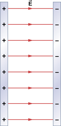

Figure 5.26 Two charged infinite planes. Note the direction of the electric field.

Strategy

We already know the electric field resulting from a single infinite plane, so we may use the principle of superposition to find the field from two.

Solution

The electric field points away from the positively charged plane and toward the negatively charged plane. Since the $\sigma$ are equal and opposite, this means that in the region outside of the two planes, the electric fields cancel each other out to zero.

However, in the region between the planes, the electric fields add, and we get

$$\overrightarrow{\text{E}}=\frac{\sigma }{{\epsilon }_0}\widehat{\text{i}}$$

for the electric field. The $\widehat{\text{i}}$ is because in the figure, the field is pointing in the +x-direction.

Significance

Systems that may be approximated as two infinite planes of this sort provide a useful means of creating uniform electric fields.