12.2 Examples of Static Equilibrium

Learning Objectives

By the end of this section, you will be able to:

Identify and analyze static equilibrium situations
Set up a free-body diagram for an extended object in static equilibrium
Set up and solve static equilibrium conditions for objects in equilibrium in various physical situations

All examples in this chapter are planar problems. Accordingly, we use equilibrium conditions in the component form of Equation 12.7 to Equation 12.9. We introduced a problem-solving strategy in Example 12.1 to illustrate the physical meaning of the equilibrium conditions. Now we generalize this strategy in a list of steps to follow when solving static equilibrium problems for extended rigid bodies. We proceed in five practical steps.

Problem-Solving Strategy

Static Equilibrium

Identify the object to be analyzed. For some systems in equilibrium, it may be necessary to consider more than one object. Identify all forces acting on the object. Identify the questions you need to answer. Identify the information given in the problem. In realistic problems, some key information may be implicit in the situation rather than provided explicitly.
Set up a free-body diagram for the object. (a) Choose the xy-reference frame for the problem. Draw a free-body diagram for the object, including only the forces that act on it. When suitable, represent the forces in terms of their components in the chosen reference frame. As you do this for each force, cross out the original force so that you do not erroneously include the same force twice in equations. Label all forces—you will need this for correct computations of net forces in the x- and y-directions. For an unknown force, the direction must be assigned arbitrarily; think of it as a ‘working direction’ or ‘suspected direction.’ The correct direction is determined by the sign that you obtain in the final solution. A plus sign $(+)$ means that the working direction is the actual direction. A minus sign $(-)$ means that the actual direction is opposite to the assumed working direction. (b) Choose the location of the rotation axis; in other words, choose the pivot point with respect to which you will compute torques of acting forces. On the free-body diagram, indicate the location of the pivot and the lever arms of acting forces—you will need this for correct computations of torques. In the selection of the pivot, keep in mind that the pivot can be placed anywhere you wish, but the guiding principle is that the best choice will simplify as much as possible the calculation of the net torque along the rotation axis.
Set up the equations of equilibrium for the object. (a) Use the free-body diagram to write a correct equilibrium condition Equation 12.7 for force components in the x-direction. (b) Use the free-body diagram to write a correct equilibrium condition Equation 12.11 for force components in the y-direction. (c) Use the free-body diagram to write a correct equilibrium condition Equation 12.9 for torques along the axis of rotation. Use Equation 12.10 to evaluate torque magnitudes and senses.
Simplify and solve the system of equations for equilibrium to obtain unknown quantities. At this point, your work involves algebra only. Keep in mind that the number of equations must be the same as the number of unknowns. If the number of unknowns is larger than the number of equations, the problem cannot be solved.
Evaluate the expressions for the unknown quantities that you obtained in your solution. Your final answers should have correct numerical values and correct physical units. If they do not, then use the previous steps to track back a mistake to its origin and correct it. Also, you may independently check for your numerical answers by shifting the pivot to a different location and solving the problem again, which is what we did in Example 12.1.

Note that setting up a free-body diagram for a rigid-body equilibrium problem is the most important component in the solution process. Without the correct setup and a correct diagram, you will not be able to write down correct conditions for equilibrium. Also note that a free-body diagram for an extended rigid body that may undergo rotational motion is different from a free-body diagram for a body that experiences only translational motion (as you saw in the chapters on Newton’s laws of motion). In translational dynamics, a body is represented as its CM, where all forces on the body are attached and no torques appear. This does not hold true in rotational dynamics, where an extended rigid body cannot be represented by one point alone. The reason for this is that in analyzing rotation, we must identify torques acting on the body, and torque depends both on the acting force and on its lever arm. Here, the free-body diagram for an extended rigid body helps us identify external torques.

Example 12.3

The Torque Balance

Three masses are attached to a uniform meter stick, as shown in Figure 12.9. The mass of the meter stick is 150.0 g and the masses to the left of the fulcrum are

m_{1} = 50.0 g

and

m_{2} = 75.0 g .

Find the mass

m_{3}

that balances the system when it is attached at the right end of the stick, and the normal reaction force at the fulcrum when the system is balanced.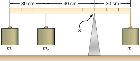

Figure is a schematic drawing of a torque balance, a horizontal beam supported at a fulcrum (indicated by S) and three masses are attached to both sides of the fulcrum. Mass 3 is 30 cm to the right of S. Mass 2 is 40 cm to the left of S. Mass 1 is 30 cm to the left of Mass 2.

Figure 12.9 In a torque balance, a horizontal beam is supported at a fulcrum (indicated by S) and masses are attached to both sides of the fulcrum. The system is in static equilibrium when the beam does not rotate. It is balanced when the beam remains level.

Strategy

For the arrangement shown in the figure, we identify the following five forces acting on the meter stick:

$w_{1} = m_{1} g$ is the weight of mass $m_{1};$ $w_{2} = m_{2} g$ is the weight of mass $m_{2};$

$w = m g$ is the weight of the entire meter stick; $w_{3} = m_{3} g$ is the weight of unknown mass $m_{3};$

$F_{S}$ is the normal reaction force at the support point S.

We choose a frame of reference where the direction of the y-axis is the direction of gravity, the direction of the x-axis is along the meter stick, and the axis of rotation (the z-axis) is perpendicular to the x-axis and passes through the support point S. In other words, we choose the pivot at the point where the meter stick touches the support. This is a natural choice for the pivot because this point does not move as the stick rotates. Now we are ready to set up the free-body diagram for the meter stick. We indicate the pivot and attach five vectors representing the five forces along the line representing the meter stick, locating the forces with respect to the pivot Figure 12.10. At this stage, we can identify the lever arms of the five forces given the information provided in the problem. For the three hanging masses, the problem is explicit about their locations along the stick, but the information about the location of the weight w is given implicitly. The key word here is “uniform.” We know from our previous studies that the CM of a uniform stick is located at its midpoint, so this is where we attach the weight w, at the 50-cm mark.

Figure is a schematic drawing of a force distribution for a torque balance, a horizontal beam supported at a fulcrum (indicated by S) and three masses are attached to both sides of the fulcrum. Force Fs at the point S is pointing upward. Force w3, to the right of point S and separated by distance r3 is pointing downward. Forces w, w2, and w1 are to the left of point S and are pointing downward. They are separated by distance r, r2, and r1, respectively.

Figure 12.10 Free-body diagram for the meter stick. The pivot is chosen at the support point S.

Solution

With Figure 12.9 and Figure 12.10 for reference, we begin by finding the lever arms of the five forces acting on the stick:

\begin{matrix} r_{1} & = & 30.0 cm + 40.0 cm = 70.0 cm \\ r_{2} & = & 40.0 cm \\ r & = & 50.0 cm - 30.0 cm = 20.0 cm \\ r_{S} & = & 0.0 cm (because F_{S} is attached at the pivot) \\ r_{3} & = & 30.0 cm. \end{matrix}

Now we can find the five torques with respect to the chosen pivot:

\begin{matrix} τ_{1} & = & + r_{1} w_{1} sin 90 ° = + r_{1} m_{1} g & (counterclockwise rotation, positive sense) \\ τ_{2} & = & + r_{2} w_{2} sin 90 ° = + r_{2} m_{2} g & (counterclockwise rotation, positive sense) \\ τ & = & + r w sin 90 ° = + r m g & (gravitational torque) \\ τ_{S} & = & r_{S} F_{S} sin θ_{S} = 0 & (because r_{S} = 0 cm) \\ τ_{3} & = & − r_{3} w_{3} sin 90 ° = − r_{3} m_{3} g & (clockwise rotation, negative sense) \end{matrix}

The second equilibrium condition (equation for the torques) for the meter stick is

τ_{1} + τ_{2} + τ + τ_{S} + τ_{3} = 0 .

When substituting torque values into this equation, we can omit the torques giving zero contributions. In this way the second equilibrium condition is

+ r_{1} m_{1} g + r_{2} m_{2} g + r m g - r_{3} m_{3} g = 0 .

12.17

Selecting the $+ y$ -direction to be parallel to ${\vec{F}}_{S},$ the first equilibrium condition for the stick is

− w_{1} - w_{2} - w + F_{S} - w_{3} = 0 .

Substituting the forces, the first equilibrium condition becomes

− m_{1} g - m_{2} g - m g + F_{S} - m_{3} g = 0 .

12.18

We solve these equations simultaneously for the unknown values $m_{3}$ and $F_{S} .$ In Equation 12.17, we cancel the g factor and rearrange the terms to obtain

r_{3} m_{3} = r_{1} m_{1} + r_{2} m_{2} + r m .

To obtain $m_{3}$ we divide both sides by $r_{3},$ so we have

\begin{matrix} m_{3} & = \frac{r_{1}}{r_{3}} m_{1} + \frac{r_{2}}{r_{3}} m_{2} + \frac{r}{r_{3}} m \\ = \frac{70}{30} (50.0 g) + \frac{40}{30} (75.0 g) + \frac{20}{30} (150.0 g) = 316.0 \frac{2}{3} g ≃ 317 g. \end{matrix}

12.19

To find the normal reaction force, we rearrange the terms in Equation 12.18, converting grams to kilograms:

\begin{matrix} F_{S} & = (m_{1} + m_{2} + m + m_{3}) g \\ = (50.0 + 75.0 + 150.0 + 316.7) \times 10^{−3} kg \times 9.8 \frac{m}{s^{2}} = 5.8 N . \end{matrix}

12.20

Significance

Notice that Equation 12.17 is independent of the value of g. The torque balance may therefore be used to measure mass, since variations in g-values on Earth’s surface do not affect these measurements. This is not the case for a spring balance because it measures the force.

Check Your Understanding 12.3

Repeat Example 12.3 using the left end of the meter stick to calculate the torques; that is, by placing the pivot at the left end of the meter stick.

In the next example, we show how to use the first equilibrium condition (equation for forces) in the vector form given by Equation 12.7 and Equation 12.8. We present this solution to illustrate the importance of a suitable choice of reference frame. Although all inertial reference frames are equivalent and numerical solutions obtained in one frame are the same as in any other, an unsuitable choice of reference frame can make the solution quite lengthy and convoluted, whereas a wise choice of reference frame makes the solution straightforward. We show this in the equivalent solution to the same problem. This particular example illustrates an application of static equilibrium to biomechanics.

Example 12.4

Forces in the Forearm

A weightlifter is holding a 50.0-lb weight (equivalent to 222.4 N) with his forearm, as shown in Figure 12.11. His forearm is positioned at

β = 60 °

with respect to his upper arm. The forearm is supported by a contraction of the biceps muscle, which causes a torque around the elbow. Assuming that the tension in the biceps acts along the vertical direction given by gravity, what tension must the muscle exert to hold the forearm at the position shown? What is the force on the elbow joint? Assume that the forearm’s weight is negligible. Give your final answers in SI units.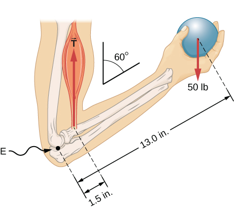

Figure is a schematic drawing of a forearm rotated around the elbow. A 50 pound ball is held in the palm. The distance between the elbow and the ball is 13 inches. The distance between the elbow and the biceps muscle, which causes a torque around the elbow, is 1.5 inches. Forearm forms a 60 degree angle with the upper arm.

Figure 12.11 The forearm is rotated around the elbow (E) by a contraction of the biceps muscle, which causes tension

{\vec{T}}_{M} .

Strategy

We identify three forces acting on the forearm: the unknown force

\vec{F}

at the elbow; the unknown tension

{\vec{T}}_{M}

in the muscle; and the weight

\vec{w}

with magnitude

w = 50 lb .

We adopt the frame of reference with the x-axis along the forearm and the pivot at the elbow. The vertical direction is the direction of the weight, which is the same as the direction of the upper arm. The x-axis makes an angle

β = 60 °

with the vertical. The y-axis is perpendicular to the x-axis. Now we set up the free-body diagram for the forearm. First, we draw the axes, the pivot, and the three vectors representing the three identified forces. Then we locate the angle

β

and represent each force by its x- and y-components, remembering to cross out the original force vector to avoid double counting. Finally, we label the forces and their lever arms. The free-body diagram for the forearm is shown in Figure 12.12. At this point, we are ready to set up equilibrium conditions for the forearm. Each force has x- and y-components; therefore, we have two equations for the first equilibrium condition, one equation for each component of the net force acting on the forearm.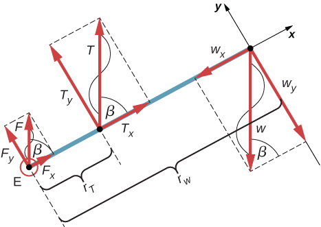

Figure is a free-body diagram for the forearm. Force F is applied at the point E. Force T is applied at the distance r tau from the point E. Force W is applied at the opposite side separated by r w from the point E. Projections of the forces at the x and y axes are shown. Forces F and T form angle beta with the x axis. Force W forms an angle beta with line connecting it with its projection to the y axis.

Figure 12.12 Free-body diagram for the forearm: The pivot is located at point E (elbow).

Notice that in our frame of reference, contributions to the second equilibrium condition (for torques) come only from the y-components of the forces because the x-components of the forces are all parallel to their lever arms, so that for any of them we have $sin θ = 0$ in Equation 12.10. For the y-components we have $θ = \pm 90 °$ in Equation 12.10. Also notice that the torque of the force at the elbow is zero because this force is attached at the pivot. So the contribution to the net torque comes only from the torques of $T_{y}$ and of $w_{y} .$

Solution

We see from the free-body diagram that the x-component of the net force satisfies the equation

+ F_{x} + T_{x} - w_{x} = 0

12.21

and the y-component of the net force satisfies

+ F_{y} + T_{y} - w_{y} = 0 .

12.22

Equation 12.21 and Equation 12.22 are two equations of the first equilibrium condition (for forces). Next, we read from the free-body diagram that the net torque along the axis of rotation is

+ r_{T} T_{y} - r_{w} w_{y} = 0 .

12.23

Equation 12.23 is the second equilibrium condition (for torques) for the forearm. The free-body diagram shows that the lever arms are $r_{T} = 1.5 in .$ and $r_{w} = 13.0 in .$ At this point, we do not need to convert inches into SI units, because as long as these units are consistent in Equation 12.23, they cancel out. Using the free-body diagram again, we find the magnitudes of the component forces:

\begin{matrix} F_{x} & = & F cos β = F cos 60 ° = F / 2 \\ T_{x} & = & T cos β = T cos 60 ° = T / 2 \\ w_{x} & = & w cos β = w cos 60 ° = w / 2 \\ F_{y} & = & F sin β = F sin 60 ° = F \sqrt{3} / 2 \\ T_{y} & = & T sin β = T sin 60 ° = T \sqrt{3} / 2 \\ w_{y} & = & w sin β = w sin 60 ° = w \sqrt{3} / 2 . \end{matrix}

We substitute these magnitudes into Equation 12.21, Equation 12.22, and Equation 12.23 to obtain, respectively,

\begin{matrix} F / 2 + T / 2 - w / 2 & = & 0 \\ F \sqrt{3} / 2 + T \sqrt{3} / 2 - w \sqrt{3} / 2 & = & 0 \\ r_{T} T \sqrt{3} / 2 - r_{w} w \sqrt{3} / 2 & = & 0 . \end{matrix}

When we simplify these equations, we see that we are left with only two independent equations for the two unknown force magnitudes, F and T, because Equation 12.21 for the x-component is equivalent to Equation 12.22 for the y-component. In this way, we obtain the first equilibrium condition for forces

F + T - w = 0

12.24

and the second equilibrium condition for torques

r_{T} T - r_{w} w = 0 .

12.25

The magnitude of tension in the muscle is obtained by solving Equation 12.25:

T = \frac{r_{w}}{r_{T}} w = \frac{13.0}{1.5} (50 lb) = 433 \frac{1}{3} lb ≃ 433.3 lb.

The force at the elbow is obtained by solving Equation 12.24:

F = w - T = 50.0 lb - 433.3 lb = −383.3 lb.

The negative sign in the equation tells us that the actual force at the elbow is antiparallel to the working direction adopted for drawing the free-body diagram. In the final answer, we convert the forces into SI units of force. The answer is

\begin{matrix} F = 383.3 lb = 383.3 (4.448 N) = 1705 N downward \\ T = 433.3 lb = 433.3 (4.448 N) = 1927 N upward. \end{matrix}

Significance

Two important issues here are worth noting. The first concerns conversion into SI units, which can be done at the very end of the solution as long as we keep consistency in units. The second important issue concerns the hinge joints such as the elbow. In the initial analysis of a problem, hinge joints should always be assumed to exert a force in an arbitrary direction, and then you must solve for all components of a hinge force independently. In this example, the elbow force happens to be vertical because the problem assumes the tension by the biceps to be vertical as well. Such a simplification, however, is not a general rule.

Solution

Suppose we adopt a reference frame with the direction of the y-axis along the 50-lb weight and the pivot placed at the elbow. In this frame, all three forces have only y-components, so we have only one equation for the first equilibrium condition (for forces). We draw the free-body diagram for the forearm as shown in Figure 12.13, indicating the pivot, the acting forces and their lever arms with respect to the pivot, and the angles

θ_{T}

and

θ_{w}

that the forces

{\vec{T}}_{M}

and

\vec{w}

(respectively) make with their lever arms. In the definition of torque given by Equation 12.10, the angle

θ_{T}

is the direction angle of the vector

{\vec{T}}_{M},

counted counterclockwise from the radial direction of the lever arm that always points away from the pivot. By the same convention, the angle

θ_{w}

is measured counterclockwise from the radial direction of the lever arm to the vector

\vec{w} .

Done this way, the non-zero torques are most easily computed by directly substituting into Equation 12.10 as follows: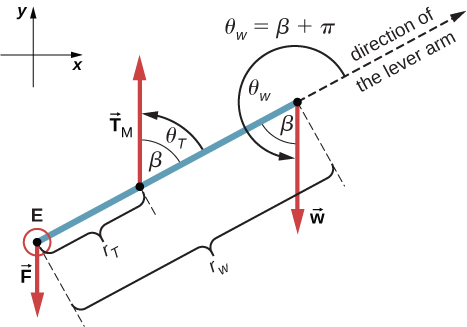

\begin{matrix} τ_{T} = r_{T} T sin θ_{T} = r_{T} T sin β = r_{T} T sin 60 ° = + r_{T} T \sqrt{3} / 2 \\ τ_{w} = r_{w} w sin θ_{w} = r_{w} w sin (β + 180 °) = − r_{w} w sin β = − r_{w} w \sqrt{3} / 2 . \end{matrix}

Figure is a free-body diagram for the forearm. Force F is applied at the point E. Force Tm is applied at the distance r tau from the point E. Force W is applied at the opposite side separated by r w from the point E. Projections of the forces at the x and y axes are shown. Force Tm forms and angle theta tau that is equal to beta with the direction of the lever arm. Force W forms an angle theta w that is equal to the sum of beta and Pi with the direction of the lever arm.

Figure 12.13 Free-body diagram for the forearm for the equivalent solution. The pivot is located at point E (elbow).

The second equilibrium condition, $τ_{T} + τ_{w} = 0,$ can be now written as

r_{T} T \sqrt{3} / 2 - r_{w} w \sqrt{3} / 2 = 0 .

12.26

From the free-body diagram, the first equilibrium condition (for forces) is

− F + T - w = 0 .

12.27

Equation 12.26 is identical to Equation 12.25 and gives the result $T = 433.3 lb .$ Equation 12.27 gives

F = T - w = 433.3 lb - 50.0 lb = 383.3 lb.

We see that these answers are identical to our previous answers, but the second choice for the frame of reference leads to an equivalent solution that is simpler and quicker because it does not require that the forces be resolved into their rectangular components.

Check Your Understanding 12.4

Repeat Example 12.4 assuming that the forearm is an object of uniform density that weighs 8.896 N.

Example 12.5

A Ladder Resting Against a Wall

A uniform ladder is

L = 5.0 m

long and weighs 400.0 N. The ladder rests against a slippery vertical wall, as shown in Figure 12.14. The minimum inclination angle between the ladder and the rough floor below which the ladder slips is

β = 53 ° .

Find the reaction forces from the floor and from the wall on the ladder and the coefficient of static friction

μ_{s}

at the interface of the ladder with the floor that prevents the ladder from slipping.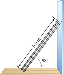

Figure is a schematic drawing of a 5.0-m-long ladder resting against a wall. Ladder forms a 53 degree angle with the floor.

Figure 12.14 A 5.0-m-long ladder rests against a frictionless wall.

Strategy

We can identify four forces acting on the ladder. The first force is the normal reaction force N from the floor in the upward vertical direction. The second force is the static friction force

f = μ_{s} N

directed horizontally along the floor toward the wall—this force prevents the ladder from slipping. These two forces act on the ladder at its contact point with the floor. The third force is the weight w of the ladder, attached at its CM located midway between its ends. The fourth force is the normal reaction force F from the wall in the horizontal direction away from the wall, attached at the contact point with the wall. There are no other forces because the wall is slippery, which means there is no friction between the wall and the ladder. Based on this analysis, we adopt the frame of reference with the y-axis in the vertical direction (parallel to the wall) and the x-axis in the horizontal direction (parallel to the floor). In this frame, each force has either a horizontal component or a vertical component but not both, which simplifies the solution. We select the pivot at the contact point with the floor. In the free-body diagram for the ladder, we indicate the pivot, all four forces and their lever arms, and the angles between lever arms and the forces, as shown in Figure 12.15. With our choice of the pivot location, there is no torque either from the normal reaction force N or from the static friction f because they both act at the pivot.

Figure is a free-body diagram for a ladder that forms an angle beta with the floor and rests against a wall. Force N is applied at the point at the floor and is perpendicular to the floor. Force W is applied at the mid-point of the ladder. Force F is applied at the point resting at the wall and is perpendicular to the wall. Force W forms an angle theta w with the direction of the lever arm. Theta w is equal to the sum of Pi and half Pi with the beta subtracted. Force F forms an angle theta F with the direction of the lever arm. Theta F is equal to the Pi minus beta.

Figure 12.15 Free-body diagram for a ladder resting against a frictionless wall.

Solution

From the free-body diagram, the net force in the x-direction is

+ f - F = 0

12.28

the net force in the y-direction is

+ N - w = 0

12.29

and the net torque along the rotation axis at the pivot point is

τ_{w} + τ_{F} = 0 .

12.30

where $τ_{w}$ is the torque of the weight w and $τ_{F}$ is the torque of the reaction F. From the free-body diagram, we identify that the lever arm of the reaction at the wall is $r_{F} = L = 5.0 m$ and the lever arm of the weight is $r_{w} = L / 2 = 2.5 m .$ With the help of the free-body diagram, we identify the angles to be used in Equation 12.10 for torques: $θ_{F} = 180 ° - β$ for the torque from the reaction force with the wall, and $θ_{w} = 180 ° + (90 ° - β)$ for the torque due to the weight. Now we are ready to use Equation 12.10 to compute torques:

\begin{matrix} τ_{w} = r_{w} w sin θ_{w} = r_{w} w sin (180 ° + 90 ° - β) = - \frac{L}{2} w sin (90 ° - β) = - \frac{L}{2} w cos β \\ τ_{F} = r_{F} F sin θ_{F} = r_{F} F sin (180 ° - β) = L F sin β . \end{matrix}

We substitute the torques into Equation 12.30 and solve for $F :$

\begin{matrix} - \frac{L}{2} w cos β + L F sin β & = & 0 \\ F = \frac{w}{2} cot β = \frac{400.0 N}{2} cot 53 ° & = & 150.7 N \end{matrix}

12.31

We obtain the normal reaction force with the floor by solving Equation 12.29: $N = w = 400.0 N .$ The magnitude of friction is obtained by solving Equation 12.28: $f = F = 150.7 N .$ Since the ladder will slip if the angle is any smaller, the static friction force is at its maximum angle and the coefficient of static friction is $μ_{s} = f / N = 150.7 / 400.0 = 0.377 .$

The net force on the ladder at the contact point with the floor is the vector sum of the normal reaction from the floor and the static friction forces:

{\vec{F}}_{floor} = \vec{f} + \vec{N} = (150.7 N) (− \hat{i}) + (400.0 N) (+ \hat{j}) = (−150.7 \hat{i} + 400.0 \hat{j}) N.

Its magnitude is

F_{floor} = \sqrt{f^{2} + N^{2}} = \sqrt{{150.7}^{2} + {400.0}^{2}} N = 427.4 N

and its direction is

φ = {tan}^{−1} (N / f) = {tan}^{−1} (400.0 / 150.7) = 69.3 ° above the floor.

We should emphasize here two general observations of practical use. First, notice that when we choose a pivot point, there is no expectation that the system will actually pivot around the chosen point. The ladder in this example is not rotating at all but firmly stands on the floor; nonetheless, its contact point with the floor is a good choice for the pivot. Second, notice when we use Equation 12.10 for the computation of individual torques, we do not need to resolve the forces into their normal and parallel components with respect to the direction of the lever arm, and we do not need to consider a sense of the torque. As long as the angle in Equation 12.10 is correctly identified—with the help of a free-body diagram—as the angle measured counterclockwise from the direction of the lever arm to the direction of the force vector, Equation 12.10 gives both the magnitude and the sense of the torque. This is because torque is the vector product of the lever-arm vector crossed with the force vector, and Equation 12.10 expresses the rectangular component of this vector product along the axis of rotation.

Significance

This result is independent of the length of the ladder because L is cancelled in the second equilibrium condition, Equation 12.31. No matter how long or short the ladder is, as long as its weight is 400 N and the angle with the floor is

53 °,

our results hold. But the ladder will slip if the net torque becomes negative in Equation 12.31. This happens for some angles when the coefficient of static friction is not great enough to prevent the ladder from slipping.

Check Your Understanding 12.5

For the situation described in Example 12.5, determine the values of the coefficient $μ_{s}$ of static friction for which the ladder starts slipping, given that $β$ is the angle that the ladder makes with the floor.

Example 12.6

Forces on Door Hinges

A swinging door that weighs

w = 400.0 N

is supported by hinges A and B so that the door can swing about a vertical axis passing through the hinges Figure 12.16. The door has a width of

b = 1.00 m,

and the door slab has a uniform mass density. The hinges are placed symmetrically at the door’s edge in such a way that the door’s weight is evenly distributed between them. The hinges are separated by distance

a = 2.00 m .

Find the forces on the hinges when the door rests half-open.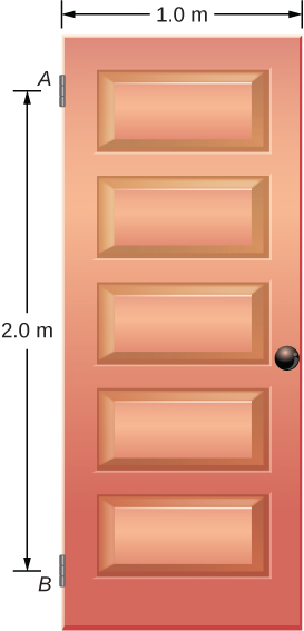

Figure is a schematic drawing of a swinging vertical door supported by two hinges attached at points A and B. The distance between points A and B is 2 meters. Door is one meter wide.

Figure 12.16 A 400-N swinging vertical door is supported by two hinges attached at points A and B.

Strategy

The forces that the door exerts on its hinges can be found by simply reversing the directions of the forces that the hinges exert on the door. Hence, our task is to find the forces from the hinges on the door. Three forces act on the door slab: an unknown force

\vec{A}

from hinge

A,

an unknown force

\vec{B}

from hinge

B,

and the known weight

\vec{w}

attached at the center of mass of the door slab. The CM is located at the geometrical center of the door because the slab has a uniform mass density. We adopt a rectangular frame of reference with the y-axis along the direction of gravity and the x-axis in the plane of the slab, as shown in panel (a) of Figure 12.17, and resolve all forces into their rectangular components. In this way, we have four unknown component forces: two components of force

\vec{A}

(A_{x}

and

A_{y}),

and two components of force

\vec{B}

(B_{x}

and

B_{y}) .

In the free-body diagram, we represent the two forces at the hinges by their vector components, whose assumed orientations are arbitrary. Because there are four unknowns

(A_{x},

B_{x},

A_{y},

and

B_{y}),

we must set up four independent equations. One equation is the equilibrium condition for forces in the x-direction. The second equation is the equilibrium condition for forces in the y-direction. The third equation is the equilibrium condition for torques in rotation about a hinge. Because the weight is evenly distributed between the hinges, we have the fourth equation,

A_{y} = B_{y} .

To set up the equilibrium conditions, we draw a free-body diagram and choose the pivot point at the upper hinge, as shown in panel (b) of Figure 12.17. Finally, we solve the equations for the unknown force components and find the forces.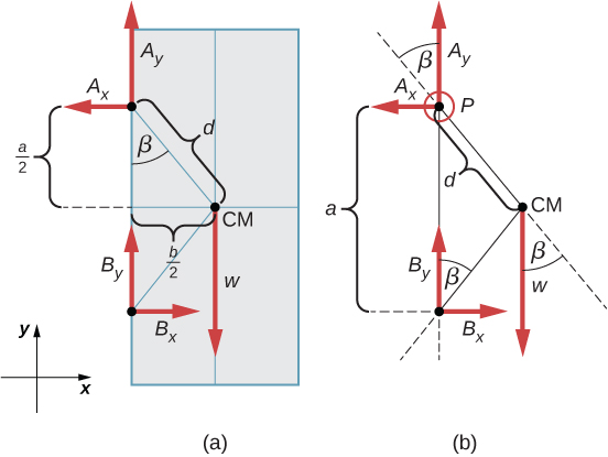

Figure A is a geometrical representation for a swinging vertical door supported by two hinges attached at points A and B. Forces A and B are applied at the points A and B. Projections of these forces to the x and y axes are shown. Force w is applied at the point CM. Point CM is lower than point A by half-a and to the right of point A by half-b. Line from point A to CM forms an angle beta with the edge of the wall. Figure B is a free-body diagram for a swinging vertical door is supported by two hinges attached at points A and B. Force Ay forms an angle beta with the line connecting points P and CM. Force By forms an angle beta with the line connecting points B and CM. Force W forms an angle beta with the line that is the continuation of the line connecting points P and CM. Distance between points P and CM is d.

Figure 12.17 (a) Geometry and (b) free-body diagram for the door.

Solution

From the free-body diagram for the door we have the first equilibrium condition for forces:

\begin{matrix} in x -direction: & - A_{x} + B_{x} = 0 \Rightarrow A_{x} = B_{x} \\ in y -direction: & + A_{y} + B_{y} - w = 0 \Rightarrow A_{y} = B_{y} = \frac{w}{2} = \frac{400.0 N}{2} = 200.0 N. \end{matrix}

We select the pivot at point P (upper hinge, per the free-body diagram) and write the second equilibrium condition for torques in rotation about point P:

pivot at P : τ_{w} + τ_{B x} + τ_{B y} = 0 .

12.32

We use the free-body diagram to find all the terms in this equation:

\begin{matrix} τ_{w} & = & d w sin (− β) = − d w sin β = − d w \frac{b / 2}{d} = − w \frac{b}{2} \\ τ_{B x} & = & a B_{x} sin 90 ° = + a B_{x} \\ τ_{B y} & = & a B_{y} sin 180 ° = 0 . \end{matrix}

In evaluating $sin β,$ we use the geometry of the triangle shown in part (a) of the figure. Now we substitute these torques into Equation 12.32 and compute $B_{x} :$

pivot at P : − w \frac{b}{2} + a B_{x} = 0 \Rightarrow B_{x} = w \frac{b}{2 a} = (400.0 N) \frac{1}{2 \cdot 2} = 100.0 N.

Therefore the magnitudes of the horizontal component forces are $A_{x} = B_{x} = 100.0 N .$ The forces on the door are

\begin{matrix} at the upper hinge: {\vec{F}}_{A on door} = −100.0 N \hat{i} + 200.0 N \hat{j} \\ at the lower hinge: {\vec{F}}_{B on door} = + 100.0 N \hat{i} + 200.0 N \hat{j} . \end{matrix}

The forces on the hinges are found from Newton’s third law as

\begin{matrix} on the upper hinge: {\vec{F}}_{door on A} = 100.0 N \hat{i} - 200.0 N \hat{j} \\ on the lower hinge: {\vec{F}}_{door on B} = −100.0 N \hat{i} - 200.0 N \hat{j} . \end{matrix}

Significance

Note that if the problem were formulated without the assumption of the weight being equally distributed between the two hinges, we wouldn’t be able to solve it because the number of the unknowns would be greater than the number of equations expressing equilibrium conditions.

Check Your Understanding 12.6

Solve the problem in Example 12.6 by taking the pivot position at the center of mass.

Check Your Understanding 12.7

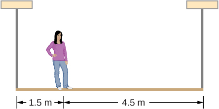
A 50-kg person stands 1.5 m away from one end of a uniform 6.0-m-long scaffold of mass 70.0 kg. Find the tensions in the two vertical ropes supporting the scaffold.

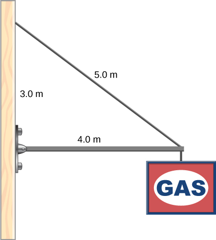
Figure is a schematic drawing of a woman standing 1.5 m away from one end and 4.5 m away from another end of a scaffold.

Check Your Understanding 12.8

A 400.0-N sign hangs from the end of a uniform strut. The strut is 4.0 m long and weighs 600.0 N. The strut is supported by a hinge at the wall and by a cable whose other end is tied to the wall at a point 3.0 m above the left end of the strut. Find the tension in the supporting cable and the force of the hinge on the strut.

Figure is a schematic drawing of a sign which hangs from the end of a uniform strut. The strut is 4.0 m long and is supported by a 5.0 m long cable tied to the wall at a point 3.0 m above the left end of the strut.